Training with DeepSpeed - Basic Concepts
basic concepts behind of DeepSpeed
Concepts of Model Parallelism
There are a few concepts that need to be reviewed: DataParallel (DP), TensorParallel (TP), PipelineParallel (PP).
DataParallel (DP)
In DP, the same setup is replicated multiple times, and each being fed a slice of the data. The processing is done in parallel and all setups are synchronized at the end of each training step.
Consider a simple model with 3 layers, where each layer has 2 params:
La | Lb | Lc
---|----|---
a0 | b0 | c0
a1 | b1 | c1
If we have two GPUs, DP splits the model onto 2 GPUs like so:
GPU0:
L0 | L1 | L2
---|----|---
a0 | b0 | c0
a1 | b1 | c1

GPU1:
L0 | L1 | L2
---|----|---
a0 | b0 | c0
a1 | b1 | c1
Each GPU holds a model, and with every iteration (step), the batch data is divided into 2 equally sized micro-batches. Each GPU independently calculates the gradients based on the micro-batch data it receives. Then the gradient is averaged by the Allreduce algorithm across all GPUs.
TensorParallel (TP)
Each tensor is split up into multiple chunks. Each shard of the tensor resides on its designated gpu. During processing each shard gets processed separately and in parallel on different GPUs and the results are synced at the end of the step. This is also called horizontal parallelism, as the splitting happens on horizontal level.
GPU0:
L0 | L1 | L2
---|----|---
a0 | b0 | c0

GPU1:
L0 | L1 | L2
---|----|---
a1 | b1 | c1
Naive Model Parallel (NMP) and PipelineParallel (PP)
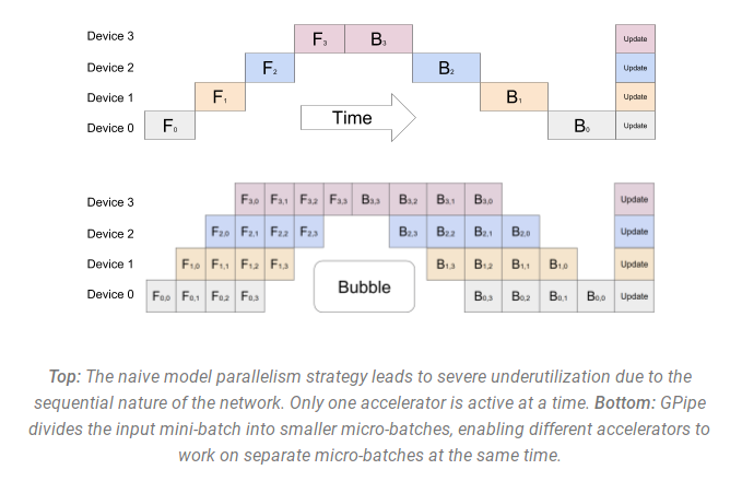
In Naive Model Parallel (MP), in comparison to data parallelism which replicates the model across GPUs, the model is instead split across its layers into multiple stages. Each stage consists of multiple layers of the model, and is placed on a different GPU. In the forward pass, the output of each stage is passed to the next stage, and the final output is the result of the last stage. This is also called vertical parallelism, as the splitting happens on vertical (layers) level.
================   =================
|  L0 | L1 | L2 |   | L3 | L4 | L5 |
=================  =================
        GPU0                 GPU1
---------------------------> forward
<--------------------------- backward
The backward pass is performed in the reverse order, starting from the last stage and ending at the first stage. This way, each GPU only requires a subset of the model, reducing the memory requirements and allowing for larger models to be trained. At the same time, we introduce minimal communication between GPUs, as the output of each stage is only passed to the next stage.
However there are two obvious problems:
- GPU utilization is not high enough, a.k.a.,
idling problem. - The outputs of each layer (activations) need to be saved and occupy a large amount of memory.
Pipeline Parallel (PP) is almost identical to a naive MP, but it solves the GPU idling problem. The idea is to split the input batch into smaller sub-batches (micro-batches), and processing them sequentially. At the end of each micro-batch, we communicate the outputs between stages, and start processing the next micro-batch. This way, we can keep the devices busy while waiting for the output of the previous stage, and reduce the pipeline bubble problem.

Compared to the original pipeline, we can see that the devices are kept busy for a larger portion of the time, as they are processing the micro-batches sequentially. However, we also note that the communication between stages is now more frequent, as we need to communicate the output of each micro-batch. This can lead to increased communication overhead, especially for small micro-batches. In practice, the choice of the micro-batch size is a trade-off between the pipeline bubble problem, the communication overhead, and the max utilization we can achieve per device with this micro-batch size.
Memory Consumption in Model Training
During model training, most of the memory is consumed by two things:
-
Model states, which includes tensors comprising of optimizer states, gradients, and model parameters. Model states are must-saved. -
Residual states, which includes any tensor that is created in the forward pass and is necessary for gradient computation during backward pass, e.g., activation, temporary buffers and unusable fragmented memory. Residual states are not necessarily saved during model training.
The state-of-the-art approach to train LLMs on the current generation of GPUs is via mixed precision.
Assume we train a model with $\Uppsi$ parameters using Adam. This requires to $2\Uppsi + 2\Uppsi + 3*4\Uppsi = 16\Uppsi$ bytes of memory requirement (see our blog Mixed-precision training in LLM for details).
Introduction to ZeRO
Challege to previous parallelism:
- DP: it does not help reduce memory footprint per device - a model with more than 1 billion parameters runs out of memory even on GPUs with 32GB of memory.
- TP/MP: it does not scale efficiently beyond a single node due to fine-grained computation and expensive communication.
ZeRO-DP
Model states often consume the largest amount of memory during training, but existing approaches such as DP and MP do not offer satisfying solution. DP has good compute/communication efficiency but poor memory efficiency while MP can have poor compute/communication efficiency.
ZeRO-DP removes the memory state redundancies across data-parallel processes by partitioning the model states instead of replicating them, and it retains the compute/communication efficiency by retaining the computational granularity and communication volume of DP using a dynamic communication schedule during training.
ZeRO-DP has three main optimization stages, which correspond to the partitioning of optimizer states, gradients, and parameters:
- Optimizer State Partitioning ($P_{os}$): 4x memory reduction, same communication volume as DP;
- Add Gradient Partitioning ($P_{os+g}$): 8x memory reduction, same communication volume as DP;
- Add Parameter Partitioning ($P_{os+g+p}$): Memory reduction is linear with DP degree Nd. For example, splitting across 64 GPUs will yield a 64x memory reduction. There is a modest 50% increase in communication volume.